Replication of Angrist and Lavy (1999)

Using maimonides’ rule to estimate the effect of class size on scholastic achievement

Author

Molly Tseng

Published

April 21, 2026

Introduction

This paper studies an important question in education:

Do smaller classes improve students’ academic performance?

Answering this question is difficult because class size is not randomly assigned. Schools with better resources or students from wealthier backgrounds may also have different class sizes, making it hard to identify causal effects.

To address this issue, the authors use a rule from Israeli schools, known as Maimonides’ rule, which sets a maximum class size of 40 students. When enrollment exceeds 40, classes are split, leading to a sudden drop in class size.

This creates a natural experiment: students in grades with 39 and 41 students are very similar, but experience very different class sizes. The authors exploit this discontinuity by using the class size predicted by the rule as an instrument for actual class size, within a regression discontinuity framework, to identify causal effects.

The results show that smaller classes significantly improve test scores for fifth graders, have a modest positive effect for fourth graders, and show little effect for third graders, likely due to data limitations.

Overall, the findings suggest that reducing class size can have meaningful benefits for student achievement, especially for older students, and highlight the importance of using credible identification strategies to estimate causal effects in education policy.

Main Analysis

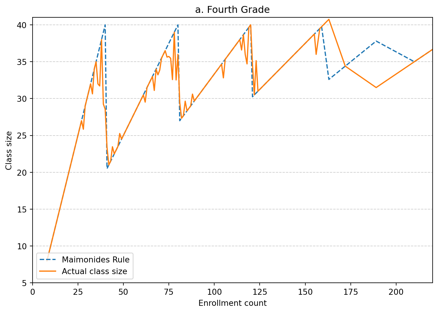
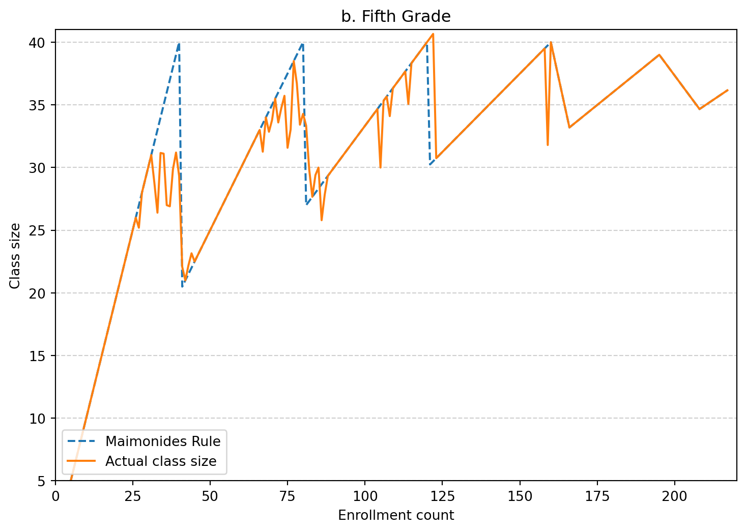
Figure 1 (4th grade) - intuition

Figure 1 shows how Maimonides’ Rule creates variation in class size based on enrollment. As enrollment increases, class size rises until it reaches 40 students. Once enrollment passes this threshold, classes are split, causing a sudden drop in average class size.

This creates a sawtooth pattern: class size increases smoothly but drops sharply at cutoffs like 40 and 80. Schools just below and above these cutoffs are very similar, except for class size.

This discontinuity provides useful variation that allows us to estimate the causal effect of class size using a regression discontinuity design.

import pandas as pd
import numpy as np
import matplotlib.pyplot as plt
import statsmodels.api as sm
df4 = pd.read_stata("/Users/mollytseng/Desktop/UCSD/quarto_website/posts/Angrist_Lavy_papers/data/dataverse_files/final4.dta")
print(df4.columns.tolist())
df4.head()

# Maimonides Rule
df4["pred_class_size"] = df4["cohsize"] / (np.floor((df4["cohsize"] - 1) / 40) + 1)

# group by enrollment
fig1_data = (
    df4.groupby("cohsize", as_index=False)
       .agg(
           actual_class_size=("classize", "mean"),
           pred_class_size=("pred_class_size", "mean")
       )
       .sort_values("cohsize")
)
print(fig1_data)

# plot
plt.figure(figsize=(9,6))

plt.plot(
    fig1_data["cohsize"],
    fig1_data["pred_class_size"],
    linestyle="--",
    label="Maimonides Rule"
)

plt.plot(
    fig1_data["cohsize"],
    fig1_data["actual_class_size"],
    linestyle="-",
    label="Actual class size"
)

plt.xlim(0, 220)
plt.ylim(5, 41)
plt.xlabel("Enrollment count")
plt.ylabel("Class size")
plt.title("a. Fourth Grade")
plt.grid(axis="y", linestyle="--", alpha=0.6)
plt.legend(loc="lower left")

plt.show()
['schlcode', 'c_size', 'c_boys', 'c_girls', 'c_numcl', 'c_pik', 'c_status', 'c_leom', 'c_tip', 'c_num4rd', 'c_type', 'flgrm4', 'mrkgrm4', 'ngrm4', 'flmth4', 'mrkmth4', 'nmth4', 'towncode', 'townname', 'popcode', 'tip_a', 'grade', 'classid', 'classize', '_type_', '_freq_', 'cohsize', 'mathsize', 'avgmath', 'passmath', 'verbsize', 'avgverb', 'passverb', 'studchk', 'misskov2', 'missagg', 'nmiss_k', 'nmiss_a', 'classct', 'math_n', 'flmath_n', 'nmath_n', 'verb_n', 'flverb_n', 'nverb_n', 'impute', 'nverb_m', 'nmath_m', 'tip_s', 'townid', 'tipuach']
     cohsize  actual_class_size  pred_class_size
0          8                8.0              8.0
1         10               10.0             10.0
2         11               11.0             11.0
3         12               12.0             12.0
4         13               13.0             13.0
..       ...                ...              ...
138      172               34.4             34.4
139      189               31.5             37.8
140      210               35.0             35.0
141      213               35.5             35.5
142      225               37.5             37.5

[143 rows x 3 columns]

Figure 1 (5th grade) - intuition

import pandas as pd
import numpy as np
import matplotlib.pyplot as plt
import statsmodels.api as sm
df5 = pd.read_stata("/Users/mollytseng/Desktop/UCSD/quarto_website/posts/Angrist_Lavy_papers/data/dataverse_files/final5.dta")
print(df5.columns.tolist())
df5.head()

# Maimonides Rule
df5["pred_class_size"] = df5["cohsize"] / (np.floor((df5["cohsize"] - 1) / 40) + 1)

# group by enrollment
fig2_data = (
    df5.groupby("cohsize", as_index=False)
       .agg(
           actual_class_size=("classize", "mean"),
           pred_class_size=("pred_class_size", "mean")
       )
       .sort_values("cohsize")
)
print(fig2_data)

# plot
plt.figure(figsize=(9,6))

plt.plot(
    fig2_data["cohsize"],
    fig2_data["pred_class_size"],
    linestyle="--",
    label="Maimonides Rule"
)

plt.plot(
    fig2_data["cohsize"],
    fig2_data["actual_class_size"],
    linestyle="-",
    label="Actual class size"
)

plt.xlim(0, 220)
plt.ylim(5, 41)
plt.xlabel("Enrollment count")
plt.ylabel("Class size")
plt.title("b. Fifth Grade")
plt.grid(axis="y", linestyle="--", alpha=0.6)
plt.legend(loc="lower left")

plt.show()
['schlcode', 'c_size', 'c_boys', 'c_girls', 'c_numcl', 'c_pik', 'c_status', 'c_leom', 'c_tip', 'c_num5rd', 'c_type', 'flgrm5', 'mrkgrm5', 'ngrm5', 'flmth5', 'mrkmth5', 'nmth5', 'towncode', 'townname', 'popcode', 'tip_a', 'grade', 'classid', 'classize', '_type_', '_freq_', 'cohsize', 'mathsize', 'avgmath', 'passmath', 'verbsize', 'avgverb', 'passverb', 'studchk', 'misskov2', 'missagg', 'nmiss_k', 'nmiss_a', 'classct', 'math_n', 'flmath_n', 'nmath_n', 'verb_n', 'flverb_n', 'nverb_n', 'impute', 'nverb_m', 'nmath_m', 'tip_s', 'townid', 'tipuach']
     cohsize  actual_class_size  pred_class_size
0          5           5.000000         5.000000
1          8           8.000000         8.000000
2          9           9.000000         9.000000
3         10          10.000000        10.000000
4         11          11.000000        11.000000
..       ...                ...              ...
140      188          37.600000        37.600000
141      189          37.800000        37.800000
142      195          39.000000        39.000000
143      208          34.666667        34.666667
144      217          36.166667        36.166667

[145 rows x 3 columns]

Table II - Naive OLS

A simple OLS regression of test scores on class size is first estimated. This shows the basic relationship between class size and student achievement in the data.

However, this estimate may be biased because class size is not randomly assigned. Schools with different class sizes may also differ in student background or other factors that affect test scores. Therefore, the OLS results reflect correlation, not necessarily a causal effect.

def run_ols(data, y, x):
    temp = data[[y] + x].dropna()
    X = sm.add_constant(temp[x])
    model = sm.OLS(temp[y], X).fit(cov_type="HC1")
    return model

# Column 7
ols_7 = run_ols(df4, "avgverb", ["classize"])

# Column 10
ols_10 = run_ols(df4, "avgmath", ["classize"])

print(ols_7.summary())
print(ols_10.summary())
                            OLS Regression Results                            
==============================================================================
Dep. Variable:                avgverb   R-squared:                       0.012
Model:                            OLS   Adj. R-squared:                  0.011
Method:                 Least Squares   F-statistic:                     20.85
Date:                Wed, 22 Apr 2026   Prob (F-statistic):           5.27e-06
Time:                        00:24:15   Log-Likelihood:                -7173.0
No. Observations:                2055   AIC:                         1.435e+04
Df Residuals:                    2053   BIC:                         1.436e+04
Df Model:                           1                                         
Covariance Type:                  HC1                                         
==============================================================================
                 coef    std err          z      P>|z|      [0.025      0.975]
------------------------------------------------------------------------------
const         68.3798      0.966     70.816      0.000      66.487      70.272
classize       0.1353      0.030      4.566      0.000       0.077       0.193
==============================================================================
Omnibus:                      144.377   Durbin-Watson:                   1.283
Prob(Omnibus):                  0.000   Jarque-Bera (JB):              207.090
Skew:                          -0.582   Prob(JB):                     1.07e-45
Kurtosis:                       4.032   Cond. No.                         151.
==============================================================================

Notes:
[1] Standard Errors are heteroscedasticity robust (HC1)
                            OLS Regression Results                            
==============================================================================
Dep. Variable:                avgmath   R-squared:                       0.024
Model:                            OLS   Adj. R-squared:                  0.023
Method:                 Least Squares   F-statistic:                     41.22
Date:                Wed, 22 Apr 2026   Prob (F-statistic):           1.69e-10
Time:                        00:24:15   Log-Likelihood:                -7353.5
No. Observations:                2055   AIC:                         1.471e+04
Df Residuals:                    2053   BIC:                         1.472e+04
Df Model:                           1                                         
Covariance Type:                  HC1                                         
==============================================================================
                 coef    std err          z      P>|z|      [0.025      0.975]
------------------------------------------------------------------------------
const         62.4545      1.057     59.081      0.000      60.383      64.526
classize       0.2111      0.033      6.420      0.000       0.147       0.276
==============================================================================
Omnibus:                       58.973   Durbin-Watson:                   1.318
Prob(Omnibus):                  0.000   Jarque-Bera (JB):               69.371
Skew:                          -0.363   Prob(JB):                     8.64e-16
Kurtosis:                       3.533   Cond. No.                         151.
==============================================================================

Notes:
[1] Standard Errors are heteroscedasticity robust (HC1)

The positive relationship is misleading. Larger classes are often found in better schools with stronger students, so higher test scores are driven by student background, not class size itself.

Table III - RDD

This step uses Maimonides’ Rule to estimate the effect of class size. Instead of relying on actual class size directly, it uses the class size predicted by the rule, which depends only on enrollment.

Because the rule creates sudden changes in class size at specific enrollment cutoffs, it provides a source of variation that is less likely to be related to student background or school quality. This makes the estimate more credible and closer to the true causal effect of class size on test scores.

def run_rf(data, y, x):
    temp = data[[y] + x].dropna()
    X = sm.add_constant(temp[x])
    model = sm.OLS(temp[y], X).fit(cov_type="HC1")
    return model

# Column (7)
rf_7 = run_rf(df4, "classize", ["pred_class_size", "tipuach"])

# Column (9)
rf_9 = run_rf(df4, "avgverb", ["pred_class_size", "tipuach"])

# Column (11)
rf_11 = run_rf(df4, "avgmath", ["pred_class_size", "tipuach"])

print("Column 7 (First Stage):")
print(rf_7.summary())

print("\nColumn 9 (Reading):")
print(rf_9.summary())

print("\nColumn 11 (Math):")
print(rf_11.summary())
Column 7 (First Stage):
                            OLS Regression Results                            
==============================================================================
Dep. Variable:               classize   R-squared:                       0.642
Model:                            OLS   Adj. R-squared:                  0.642
Method:                 Least Squares   F-statistic:                     1701.
Date:                Wed, 22 Apr 2026   Prob (F-statistic):               0.00
Time:                        00:24:15   Log-Likelihood:                -5687.8
No. Observations:                2059   AIC:                         1.138e+04
Df Residuals:                    2056   BIC:                         1.140e+04
Df Model:                           2                                         
Covariance Type:                  HC1                                         
===================================================================================
                      coef    std err          z      P>|z|      [0.025      0.975]
-----------------------------------------------------------------------------------
const               4.7264      0.540      8.754      0.000       3.668       5.785
pred_class_size     0.8460      0.017     49.561      0.000       0.813       0.880
tipuach            -0.0342      0.007     -4.925      0.000      -0.048      -0.021
==============================================================================
Omnibus:                      995.114   Durbin-Watson:                   1.594
Prob(Omnibus):                  0.000   Jarque-Bera (JB):            18558.350
Skew:                          -1.820   Prob(JB):                         0.00
Kurtosis:                      17.250   Cond. No.                         201.
==============================================================================

Notes:
[1] Standard Errors are heteroscedasticity robust (HC1)

Column 9 (Reading):
                            OLS Regression Results                            
==============================================================================
Dep. Variable:                avgverb   R-squared:                       0.312
Model:                            OLS   Adj. R-squared:                  0.311
Method:                 Least Squares   F-statistic:                     335.3
Date:                Wed, 22 Apr 2026   Prob (F-statistic):          9.71e-127
Time:                        00:24:15   Log-Likelihood:                -6800.9
No. Observations:                2055   AIC:                         1.361e+04
Df Residuals:                    2052   BIC:                         1.362e+04
Df Model:                           2                                         
Covariance Type:                  HC1                                         
===================================================================================
                      coef    std err          z      P>|z|      [0.025      0.975]
-----------------------------------------------------------------------------------
const              80.1547      0.838     95.641      0.000      78.512      81.797
pred_class_size    -0.0953      0.025     -3.784      0.000      -0.145      -0.046
tipuach            -0.3423      0.013    -25.891      0.000      -0.368      -0.316
==============================================================================
Omnibus:                      100.621   Durbin-Watson:                   1.424
Prob(Omnibus):                  0.000   Jarque-Bera (JB):              153.215
Skew:                          -0.424   Prob(JB):                     5.37e-34
Kurtosis:                       4.034   Cond. No.                         202.
==============================================================================

Notes:
[1] Standard Errors are heteroscedasticity robust (HC1)

Column 11 (Math):
                            OLS Regression Results                            
==============================================================================
Dep. Variable:                avgmath   R-squared:                       0.201
Model:                            OLS   Adj. R-squared:                  0.201
Method:                 Least Squares   F-statistic:                     215.8
Date:                Wed, 22 Apr 2026   Prob (F-statistic):           8.56e-86
Time:                        00:24:15   Log-Likelihood:                -7146.9
No. Observations:                2055   AIC:                         1.430e+04
Df Residuals:                    2052   BIC:                         1.432e+04
Df Model:                           2                                         
Covariance Type:                  HC1                                         
===================================================================================
                      coef    std err          z      P>|z|      [0.025      0.975]
-----------------------------------------------------------------------------------
const              72.1936      1.082     66.738      0.000      70.073      74.314
pred_class_size     0.0229      0.032      0.705      0.481      -0.041       0.087
tipuach            -0.2923      0.014    -20.301      0.000      -0.320      -0.264
==============================================================================
Omnibus:                       49.922   Durbin-Watson:                   1.382
Prob(Omnibus):                  0.000   Jarque-Bera (JB):               66.047
Skew:                          -0.284   Prob(JB):                     4.55e-15
Kurtosis:                       3.670   Cond. No.                         202.
==============================================================================

Notes:
[1] Standard Errors are heteroscedasticity robust (HC1)

Comparison

Comparing the naive OLS and reduced-form estimates, the results change both in magnitude and sign. The OLS estimates suggest a positive relationship between class size and test scores, implying that larger classes are associated with better performance. However, this result is likely driven by selection bias.

In contrast, the reduced-form estimates based on Maimonides’ Rule show a negative relationship between class size and reading scores. This suggests that larger classes actually reduce student achievement once more credible variation is used.

The key difference is that the OLS estimates capture correlations influenced by student background and school characteristics, while the reduced-form approach isolates variation in class size that is driven by enrollment rules. As a result, the reduced-form estimates provide a more reliable indication of the causal effect of class size.

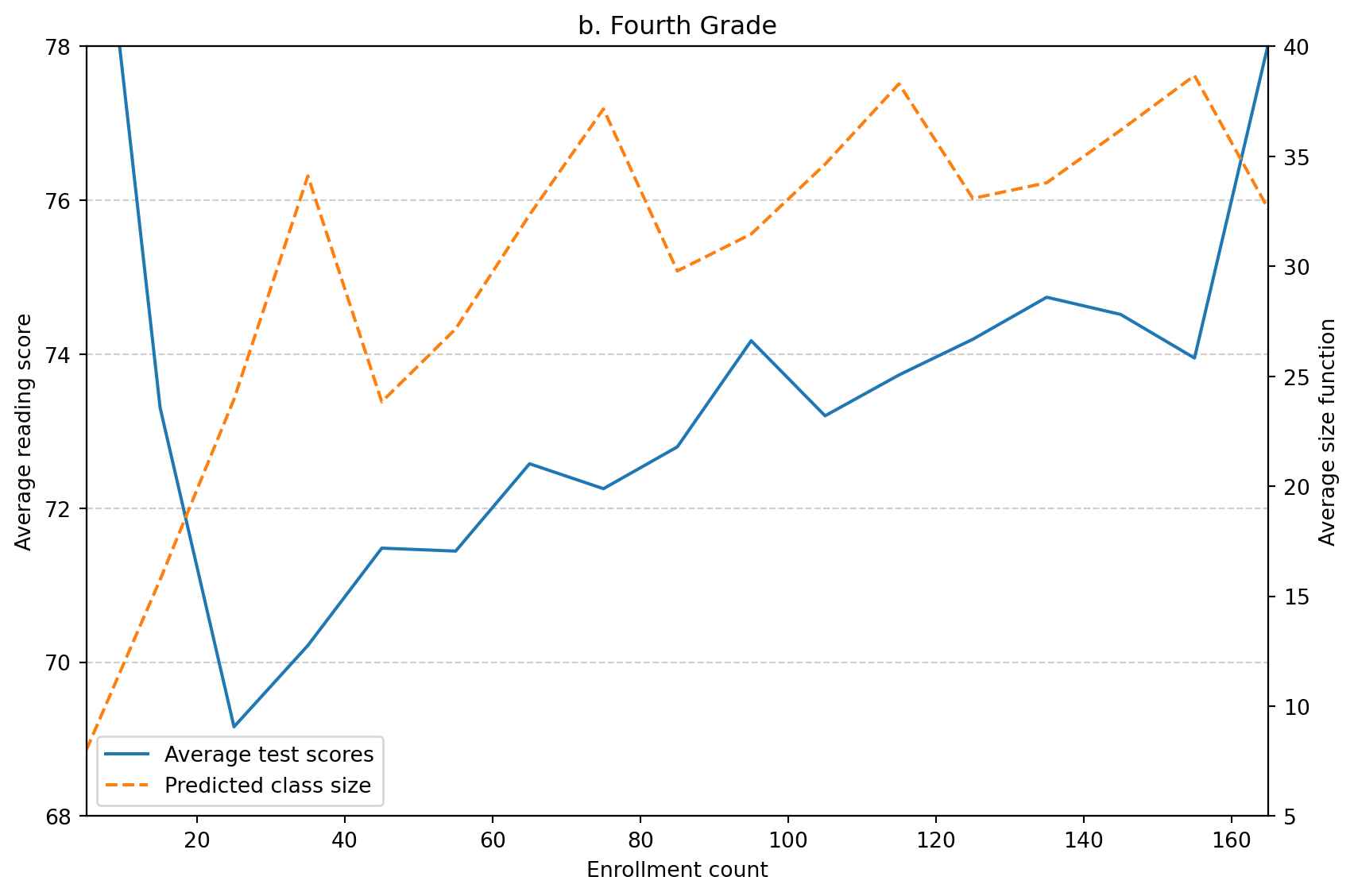
Something Additional

As an additional analysis, I plot average reading scores against enrollment to provide a visual complement to the regression results.

The pattern appears to move in the opposite direction of class size. When enrollment crosses thresholds such as 40 or 80, class size drops, and test scores tend to increase. This mirrors the pattern observed in Figure 1.

# create enrollment bins (each 10 per bins)
df4["enroll_bin"] = (df4["cohsize"] // 10) * 10

fig2_data = (
    df4.groupby("enroll_bin", as_index=False)
       .agg(
           avg_reading=("avgverb", "mean"),
           pred_class_size=("pred_class_size", "mean")
       )
       .sort_values("enroll_bin")
)
# add midpoint for x-axis
fig2_data["x_mid"] = fig2_data["enroll_bin"] + 5

fig, ax1 = plt.subplots(figsize=(9,6))

# reading score
ax1.plot(
    fig2_data["x_mid"],
    fig2_data["avg_reading"],
    linestyle="-",
    color="tab:blue",
    label="Average test scores"
)

ax1.set_xlabel("Enrollment count")
ax1.set_ylabel("Average reading score")
ax1.set_xlim(5, 165)
ax1.set_ylim(68, 78)

# predicted class size
ax2 = ax1.twinx()

ax2.plot(
    fig2_data["x_mid"],
    fig2_data["pred_class_size"],
    linestyle="--",
    color="tab:orange",
    label="Predicted class size"
)

ax2.set_ylabel("Average size function")
ax2.set_ylim(5, 40)

# legend
lines1, labels1 = ax1.get_legend_handles_labels()
lines2, labels2 = ax2.get_legend_handles_labels()
ax1.legend(lines1 + lines2, labels1 + labels2, loc="lower left")

ax1.grid(axis="y", linestyle="--", alpha=0.6)
plt.title("b. Fourth Grade")

plt.tight_layout()
plt.show()

Conclusion

Using Maimonides’ Rule, this paper finds that smaller class sizes improve student achievement, particularly in reading. While naive OLS results are biased, the regression discontinuity approach provides more credible evidence of a negative causal effect of class size.

Reference

Angrist, J. D., & Lavy, V. (1999). Using Maimonides’ Rule to Estimate the Effect of Class Size on Scholastic Achievement